Note
Click here to download the full example code
Plot R-squared for a linear model
# Authors: Jose C. Garcia Alanis <alanis.jcg@gmail.com>
#
# License: BSD (3-clause)

import numpy as np

from sklearn.linear_model import LinearRegression
from sklearn.metrics import r2_score

from mne.decoding import Vectorizer, get_coef
from mne.datasets import limo
from mne.evoked import EvokedArray
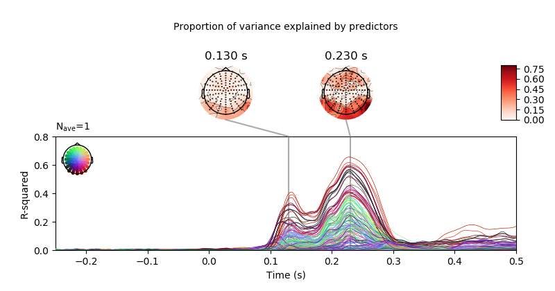
Here, we’ll import only one subject. The example shows how to calculate the coefficient of determination (R-squared) for a liner model fitted wit sklearn, showing where (i.e., which electrodes) and when (i.e., at what time of the analysis time window) the model fit best to the data.
# subject id
subjects = [2]
# create a dictionary containing participants data
limo_epochs = {str(subj): limo.load_data(subject=subj) for subj in subjects}

# interpolate missing channels
for subject in limo_epochs.values():
    subject.interpolate_bads(reset_bads=True)

# epochs to use for analysis
epochs = limo_epochs['2']

# only keep eeg channels
epochs = epochs.pick_types(eeg=True)

# save epochs information (needed for creating a homologous
# epochs object containing linear regression result)
epochs_info = epochs.info
tmin = epochs.tmin
Out:
1052 matching events found
No baseline correction applied
Adding metadata with 2 columns
0 projection items activated
0 bad epochs dropped
Computing interpolation matrix from 117 sensor positions
Interpolating 11 sensors
use epochs metadata to create design matrix for linear regression analyses
# add intercept
design = epochs.metadata.copy().assign(intercept=1)
# effect code contrast for categorical variable (i.e., condition a vs. b)
design['face a - face b'] = np.where(design['face'] == 'A', 1, -1)
# create design matrix with named predictors
predictors = ['intercept', 'face a - face b', 'phase-coherence']
design = design[predictors]
extract the data that will be used in the analyses
# get epochs data
data = epochs.get_data()

# number of epochs in data set
n_epochs = data.shape[0]

# number of channels and number of time points in each epoch
# we'll use this information later to bring the results of the
# the linear regression algorithm into an eeg-like format
# (i.e., channels x times points)
n_channels = data.shape[1]
n_times = len(epochs.times)

# vectorize (channel) data for linear regression
Y = Vectorizer().fit_transform(data)
fit linear model with sklearn
# set up model and fit linear model
linear_model = LinearRegression(fit_intercept=False)
linear_model.fit(design, Y)

# extract the coefficients for linear model estimator
betas = get_coef(linear_model, 'coef_')

# calculate coefficient of determination (r-squared)
r_squared = r2_score(Y, linear_model.predict(design), multioutput='raw_values')
# project r-squared back to channels by times space
r_squared = r_squared.reshape((n_channels, n_times))
r_squared = EvokedArray(r_squared, epochs_info, tmin)
plot model r-squared
# only show -250 to 500 ms
ts_args = dict(xlim=(-.25, 0.5),
               unit=False,
               ylim=dict(eeg=[0, 0.8]))
topomap_args = dict(cmap='Reds', scalings=dict(eeg=1),
                    vmin=0, vmax=0.8, average=0.05)
# create plot
fig = r_squared.plot_joint(ts_args=ts_args,
                           topomap_args=topomap_args,
                           title='Proportion of variance explained by '
                                 'predictors',
                           times=[.13, .23])
fig.axes[0].set_ylabel('R-squared')

Total running time of the script: ( 0 minutes 3.580 seconds)