Note
Click here to download the full example code
Plot p-values for single subject beta coefficients
References
| [1] | Sander Greenland (2019) Valid P-Values Behave Exactly as They Should: Some Misleading Criticisms of P-Values and Their Resolution With S-Values, The American Statistician, 73:sup1, https://doi.org/10.1080/00031305.2018.1543137 |
# Authors: Jose C. Garcia Alanis <alanis.jcg@gmail.com>
#
# License: BSD (3-clause)

import numpy as np
from scipy import stats
import matplotlib.pyplot as plt

from sklearn.linear_model import LinearRegression

from mne.decoding import Vectorizer, get_coef
from mne.datasets import limo
from mne.evoked import EvokedArray
from mne.stats import fdr_correction
from mne.viz import plot_compare_evokeds
Here, we’ll import only one subject. The example shows how to compute p-values for beta coefficients derived from linear regression using sklearn. In addition, we propose to visualize these p-values in terms of Shannon information values [1] (i.e., surprise values) for better interpretation.
# subject id
subjects = [2]
# create a dictionary containing participants data
limo_epochs = {str(subj): limo.load_data(subject=subj) for subj in subjects}

# interpolate missing channels
for subject in limo_epochs.values():
    subject.interpolate_bads(reset_bads=True)

# epochs to use for analysis
epochs = limo_epochs['2']

# only keep eeg channels
epochs = epochs.pick_types(eeg=True)

# save epochs information (needed for creating a homologous
# epochs object containing linear regression result)
epochs_info = epochs.info
tmin = epochs.tmin
Out:
1052 matching events found
No baseline correction applied
Adding metadata with 2 columns
0 projection items activated
0 bad epochs dropped
Computing interpolation matrix from 117 sensor positions
Interpolating 11 sensors
use epochs metadata to create design matrix for linear regression analyses
# add intercept
design = epochs.metadata.copy().assign(intercept=1)
# effect code contrast for categorical variable (i.e., condition a vs. b)
design['face a - face b'] = np.where(design['face'] == 'A', 1, -1)
# create design matrix with named predictors
predictors = ['intercept', 'face a - face b', 'phase-coherence']
design = design[predictors]
extract the data that will be used in the analyses
# get epochs data
data = epochs.get_data()

# number of epochs in data set
n_epochs = data.shape[0]

# number of channels and number of time points in each epoch
# we'll use this information later to bring the results of the
# the linear regression algorithm into an eeg-like format
# (i.e., channels x times points)
n_channels = data.shape[1]
n_times = len(epochs.times)

# number of trials and number of predictors
n_trials, n_predictors = design.shape
# degrees of freedom
dfs = float(n_trials - n_predictors)

# vectorize (channel) data for linear regression
Y = Vectorizer().fit_transform(data)
fit linear model with sklearn
# set up model and fit linear model
linear_model = LinearRegression(fit_intercept=False)
linear_model.fit(design, Y)

# extract the coefficients for linear model estimator
betas = get_coef(linear_model, 'coef_')

# compute predictions
predictions = linear_model.predict(design)

# compute sum of squared residuals and mean squared error
residuals = (Y - predictions)
# sum of squared residuals
ssr = np.sum(residuals ** 2, axis=0)
# mean squared error
sqrt_mse = np.sqrt(ssr / dfs)

# raw error terms for each predictor in the design matrix:
# here, we take the inverse of the design matrix's projections
# (i.e., A^T*A)^-1 and extract the square root of the diagonal values.
error_terms = np.sqrt(np.diag(np.linalg.pinv(np.dot(design.T, design))))
extract betas for each predictor in design matrix and compute p-values
# place holders for results
lm_betas, stderrs, t_vals, p_vals, s_vals = (dict() for _ in range(5))
# define point asymptotic to zero to use as zero
tiny = np.finfo(np.float64).tiny
# loop through predictors to extract parameters
for ind, predictor in enumerate(predictors):
# extract coefficients for predictor in question
beta = betas[:, ind]
# compute standard errors
stderr = sqrt_mse * error_terms[ind]
# compute t values
t_val = beta / stderr
# and p-values
p_val = 2 * stats.t.sf(np.abs(t_val), dfs)
# project results back to channels x time points space
beta = beta.reshape((n_channels, n_times))
stderr = stderr.reshape((n_channels, n_times))
t_val = t_val.reshape((n_channels, n_times))
# replace p-values == 0 with asymptotic value `tiny`
p_val = np.clip(p_val, tiny, 1.).reshape((n_channels, n_times))
# create evoked object for plotting
lm_betas[predictor] = EvokedArray(beta, epochs_info, tmin)
stderrs[predictor] = EvokedArray(stderr, epochs_info, tmin)
t_vals[predictor] = EvokedArray(t_val, epochs_info, tmin)
p_vals[predictor] = p_val
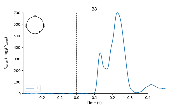
# For better interpretation, we'll transform p-values to
# Shannon information values (i.e., surprise values) by taking the
# negative log2 of the p-value. In contrast to the p-value, the resulting
# "s-value" is not a probability. Rather, it constitutes a continuous
# measure of information (in bits) against the test hypothesis (see [1]
# above for further details).
s_vals[predictor] = EvokedArray(-np.log2(p_val) * 1e-6, epochs_info, tmin)
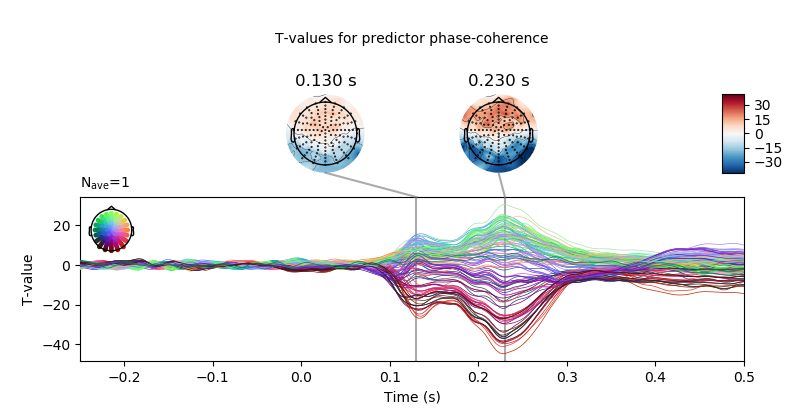
plot inference results for predictor “phase-coherence”
predictor = 'phase-coherence'

# only show -250 to 500 ms
ts_args = dict(xlim=(-.25, 0.5),
               # use unit=False to avoid conversion to micro-volt
               unit=False)
topomap_args = dict(cmap='RdBu_r',
                    # keep values scale
                    scalings=dict(eeg=1),
                    average=0.05)
# plot t-values
fig = t_vals[predictor].plot_joint(ts_args=ts_args,
                                   topomap_args=topomap_args,
                                   title='T-values for predictor ' + predictor,
                                   times=[.13, .23])
fig.axes[0].set_ylabel('T-value')
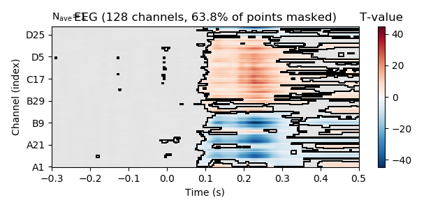
correct p-values for multiple testing and create a mask for non-significant time point dor each channel.
reject_H0, fdr_pvals = fdr_correction(p_vals[predictor],
                                      alpha=0.01)
# plot t-values, masking non-significant time points.
fig = t_vals[predictor].plot_image(time_unit='s',
                                   mask=reject_H0,
                                   unit=False,
                                   # keep values scale
                                   scalings=dict(eeg=1))
fig.axes[1].set_title('T-value')
plot surprise-values as “erp” only show electrode B8
pick = epochs.info['ch_names'].index('B8')
fig, ax = plt.subplots(figsize=(7, 4))
plot_compare_evokeds(s_vals[predictor],
                     picks=pick,
                     legend='lower left',
                     axes=ax,
                     show_sensors='upper left')
plt.rcParams.update({'mathtext.default':  'regular'})
ax.set_ylabel('$S_{value}$ (-$log_2$($P_{value}$)')
ax.yaxis.set_label_coords(-0.1, 0.5)
plt.plot()
Total running time of the script: ( 0 minutes 3.817 seconds)