Plot bootstrapped confidence interval for linear model fit¶

# Authors: Jose C. Garcia Alanis <alanis.jcg@gmail.com>
#
# License: BSD (3-clause)

import numpy as np
import matplotlib.pyplot as plt

from sklearn.linear_model import LinearRegression

from mne.viz import plot_compare_evokeds
from mne.decoding import Vectorizer, get_coef
from mne.datasets import limo
from mne.evoked import EvokedArray

# subject id
subjects = [2]

# create a dictionary containing participants data
limo_epochs = {str(subj): limo.load_data(subject=subj) for subj in subjects}

# interpolate missing channels
for subject in limo_epochs.values():
    subject.interpolate_bads(reset_bads=True)

# epochs to use for analysis
epochs = limo_epochs['2']

# only keep eeg channels
epochs = epochs.pick_types(eeg=True)

# save epochs information (needed for creating a homologous
# epochs object containing linear regression result)
epochs_info = epochs.info
tmin = epochs.tmin

# add intercept
design = epochs.metadata.copy().assign(intercept=1)
# effect code contrast for categorical variable (i.e., condition a vs. b)
design['face a - face b'] = np.where(design['face'] == 'A', 1, -1)
# create design matrix with named predictors
predictors = ['intercept', 'face a - face b', 'phase-coherence']
design = design[predictors]

# get epochs data
data = epochs.get_data()

# number of epochs in data set
n_epochs = data.shape[0]

# number of channels and number of time points in each epoch
# we'll use this information later to bring the results of the
# the linear regression algorithm into an eeg-like format
# (i.e., channels x times points)
n_channels = data.shape[1]
n_times = len(epochs.times)

# vectorize (channel) data for linear regression
Y = Vectorizer().fit_transform(data)

# set random state for replication
random_state = 42
random = np.random.RandomState(random_state)

# number of random samples
boot = 2000

# create empty array for saving the bootstrap samples
boot_betas = np.zeros((boot, Y.shape[1], len(predictors)))
# run bootstrap for regression coefficients
for i in range(boot):
    # extract random epochs from data
    resamples = random.choice(range(n_epochs), n_epochs, replace=True)
    # set up model and fit model
    model = LinearRegression(fit_intercept=False)
    model.fit(X=design.iloc[resamples], y=Y[resamples, :])
    # extract regression coefficients
    boot_betas[i, :, :] = get_coef(model, 'coef_')
    # delete the previously fitted model
    del model

lower, upper = np.quantile(boot_betas, [.025, .975], axis=0)

# set up linear model
linear_model = LinearRegression(fit_intercept=False)
# fit model
linear_model.fit(design, Y)

# extract the coefficients for linear model estimator
betas = get_coef(linear_model, 'coef_')

# project coefficients back to a channels x time points space.
lm_betas = dict()
ci = dict(lower_bound=dict(), upper_bound=dict())
# loop through predictors
for ind, predictor in enumerate(predictors):
    # extract coefficients and CI for predictor in question
    # and project back to channels x time points
    beta = betas[:, ind].reshape((n_channels, n_times))
    lower_bound = lower[:, ind].reshape((n_channels, n_times))
    upper_bound = upper[:, ind].reshape((n_channels, n_times))
    # create evoked object containing the back projected coefficients
    # for each predictor
    lm_betas[predictor] = EvokedArray(beta, epochs_info, tmin)
    # dictionary containing upper and lower confidence boundaries
    ci['lower_bound'][predictor] = lower_bound
    ci['upper_bound'][predictor] = upper_bound

# only show -250 to 500 ms
ts_args = dict(xlim=(-.25, 0.5))

# predictor to plot
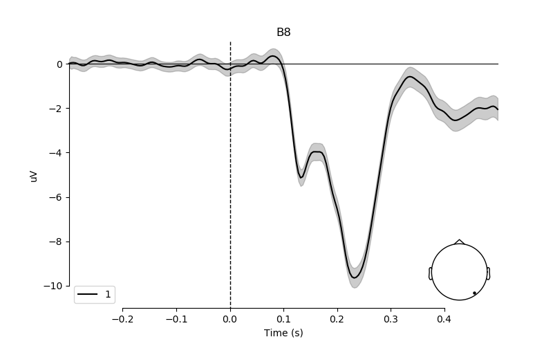
predictor = 'phase-coherence'
# electrode to plot
pick = epochs.info['ch_names'].index('B8')

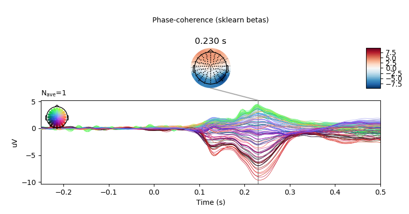
# visualise effect of phase-coherence for sklearn estimation method.
lm_betas[predictor].plot_joint(ts_args=ts_args,
                               title='Phase-coherence (sklearn betas)',
                               times=[.23])

# create plot for the effect of phase-coherence on electrode B8
# with 95% confidence interval
fig, ax = plt.subplots(figsize=(8, 5))
plot_compare_evokeds(lm_betas[predictor],
                     picks=pick,
                     ylim=dict(eeg=[-11, 1]),
                     colors=['k'],
                     legend='lower left',
                     axes=ax)
ax.fill_between(epochs.times,
                ci['lower_bound'][predictor][pick]*1e6,
                ci['upper_bound'][predictor][pick]*1e6,
                color=['k'],
                alpha=0.2)
plt.plot()