Note
Click here to download the full example code
Plot spatiotemporal clustering results for effect of continuous variable
# Authors: Jose C. Garcia Alanis <alanis.jcg@gmail.com>
#
# License: BSD (3-clause)

import numpy as np
import matplotlib.pyplot as plt

from mpl_toolkits.axes_grid1 import make_axes_locatable

from sklearn.linear_model import LinearRegression

from mne.stats.cluster_level import _setup_connectivity, _find_clusters, \
    _reshape_clusters
from mne.channels import find_ch_connectivity
from mne.datasets import limo
from mne.decoding import Vectorizer, get_coef
from mne.evoked import EvokedArray
from mne.viz import plot_topomap, plot_compare_evokeds, tight_layout
from mne import combine_evoked, find_layout
Here, we’ll import multiple subjects from the LIMO-dataset and compute group-level beta-coefficients for a continuous predictor, in addition we show how confidence (or significance) levels can be computed for this effects using the bootstrap-t technique and spatiotemporal clustering
# list with subjects ids that should be imported
subjects = list(range(1, 19))
# create a dictionary containing participants data for easy slicing
limo_epochs = {str(subj): limo.load_data(subject=subj) for subj in subjects}

# interpolate missing channels
for subject in limo_epochs.values():
    subject.interpolate_bads(reset_bads=True)
    subject = subject.crop(tmin=0, tmax=0.35)
    # only keep eeg channels
    subject.pick_types(eeg=True)
Out:
1055 matching events found
No baseline correction applied
Adding metadata with 2 columns
0 projection items activated
0 bad epochs dropped
1052 matching events found
No baseline correction applied
Adding metadata with 2 columns
0 projection items activated
0 bad epochs dropped
1072 matching events found
No baseline correction applied
Adding metadata with 2 columns
0 projection items activated
0 bad epochs dropped
1050 matching events found
No baseline correction applied
Adding metadata with 2 columns
0 projection items activated
0 bad epochs dropped
1118 matching events found
No baseline correction applied
Adding metadata with 2 columns
0 projection items activated
0 bad epochs dropped
1108 matching events found
No baseline correction applied
Adding metadata with 2 columns
0 projection items activated
0 bad epochs dropped
1060 matching events found
No baseline correction applied
Adding metadata with 2 columns
0 projection items activated
0 bad epochs dropped
1030 matching events found
No baseline correction applied
Adding metadata with 2 columns
0 projection items activated
0 bad epochs dropped
1059 matching events found
No baseline correction applied
Adding metadata with 2 columns
0 projection items activated
0 bad epochs dropped
1038 matching events found
No baseline correction applied
Adding metadata with 2 columns
0 projection items activated
0 bad epochs dropped
1029 matching events found
No baseline correction applied
Adding metadata with 2 columns
0 projection items activated
0 bad epochs dropped
943 matching events found
No baseline correction applied
Adding metadata with 2 columns
0 projection items activated
0 bad epochs dropped
1108 matching events found
No baseline correction applied
Adding metadata with 2 columns
0 projection items activated
0 bad epochs dropped
998 matching events found
No baseline correction applied
Adding metadata with 2 columns
0 projection items activated
0 bad epochs dropped
1076 matching events found
No baseline correction applied
Adding metadata with 2 columns
0 projection items activated
0 bad epochs dropped
1061 matching events found
No baseline correction applied
Adding metadata with 2 columns
0 projection items activated
0 bad epochs dropped
1098 matching events found
No baseline correction applied
Adding metadata with 2 columns
0 projection items activated
0 bad epochs dropped
1103 matching events found
No baseline correction applied
Adding metadata with 2 columns
0 projection items activated
0 bad epochs dropped
Computing interpolation matrix from 113 sensor positions
Interpolating 15 sensors
Computing interpolation matrix from 117 sensor positions
Interpolating 11 sensors
Computing interpolation matrix from 121 sensor positions
Interpolating 7 sensors
Computing interpolation matrix from 119 sensor positions
Interpolating 9 sensors
Computing interpolation matrix from 122 sensor positions
Interpolating 6 sensors
Computing interpolation matrix from 118 sensor positions
Interpolating 10 sensors
Computing interpolation matrix from 117 sensor positions
Interpolating 11 sensors
Computing interpolation matrix from 117 sensor positions
Interpolating 11 sensors
Computing interpolation matrix from 121 sensor positions
Interpolating 7 sensors
Computing interpolation matrix from 116 sensor positions
Interpolating 12 sensors
/home/josealanis/Documents/github/mne-stats/examples/group_level/plot_spatiotemporal_cluster.py:41: RuntimeWarning: No bad channels to interpolate. Doing nothing...
  subject.interpolate_bads(reset_bads=True)
Computing interpolation matrix from 115 sensor positions
Interpolating 13 sensors
Computing interpolation matrix from 122 sensor positions
Interpolating 6 sensors
Computing interpolation matrix from 114 sensor positions
Interpolating 14 sensors
Computing interpolation matrix from 117 sensor positions
Interpolating 11 sensors
Computing interpolation matrix from 125 sensor positions
Interpolating 3 sensors
Computing interpolation matrix from 126 sensor positions
Interpolating 2 sensors
Computing interpolation matrix from 122 sensor positions
Interpolating 6 sensors
regression parameters
# variables to be used in the analysis (i.e., predictors)
predictors = ['intercept', 'face a - face b', 'phase-coherence']

# number of predictors
n_predictors = len(predictors)

# save epochs information (needed for creating a homologous
# epochs object containing linear regression result)
epochs_info = limo_epochs[str(subjects[0])].info

# number of channels and number of time points in each epoch
# we'll use this information later to bring the results of the
# the linear regression algorithm into an eeg-like format
# (i.e., channels x times points)
n_channels = len(epochs_info['ch_names'])
n_times = len(limo_epochs[str(subjects[0])].times)

# also save times first time-point in data
times = limo_epochs[str(subjects[0])].times
tmin = limo_epochs[str(subjects[0])].tmin
create empty objects for the storage of results
# place holders for bootstrap samples
betas = np.zeros((len(limo_epochs.values()),
                  n_channels * n_times))

# dicts for results evoked-objects
betas_evoked = dict()
t_evokeds = dict()
run regression analysis for each subject
# loop through subjects, set up and fit linear model
for iteration, subject in enumerate(limo_epochs.values()):

    # --- 1) create design matrix ---
    # use epochs metadata
    design = subject.metadata.copy()

    # add intercept (constant) to design matrix
    design = design.assign(intercept=1)

    # effect code contrast for categorical variable (i.e., condition a vs. b)
    design['face a - face b'] = np.where(design['face'] == 'A', 1, -1)

    # order columns of design matrix
    design = design[predictors]

    # column of betas array (i.e., predictor) to run bootstrap on
    pred_col = predictors.index('phase-coherence')

    # --- 2) vectorize (eeg-channel) data for linear regression analysis ---
    # data to be analysed
    data = subject.get_data()

    # vectorize data across channels
    Y = Vectorizer().fit_transform(data)

    # --- 3) fit linear model with sklearn's LinearRegression ---
    # we already have an intercept column in the design matrix,
    # thus we'll call LinearRegression with fit_intercept=False
    linear_model = LinearRegression(fit_intercept=False)
    linear_model.fit(design, Y)

    # --- 4) extract the resulting coefficients (i.e., betas) ---
    # extract betas
    coefs = get_coef(linear_model, 'coef_')
    # only keep relevant predictor
    betas[iteration, :] = coefs[:, pred_col]

    # the matrix of coefficients has a shape of number of observations in
    # the vertorized channel data by number of predictors;
    # thus, we can loop through the columns i.e., the predictors)
    # of the coefficient matrix and extract coefficients for each predictor
    # in order to project them back to a channels x time points space.
    lm_betas = dict()

    # extract coefficients
    beta = betas[iteration, :]
    # back projection to channels x time points
    beta = beta.reshape((n_channels, n_times))
    # create evoked object containing the back projected coefficients
    lm_betas['phase-coherence'] = EvokedArray(beta, epochs_info, tmin)

    # save results
    betas_evoked[str(subjects[iteration])] = lm_betas

    # clean up
    del linear_model
compute mean beta-coefficient for predictor phase-coherence
# subject ids
subjects = [str(subj) for subj in subjects]

# extract phase-coherence betas for each subject
phase_coherence = [betas_evoked[subj]['phase-coherence'] for subj in subjects]

# average phase-coherence betas
weights = np.repeat(1 / len(phase_coherence), len(phase_coherence))
ga_phase_coherence = combine_evoked(phase_coherence, weights=weights)
compute bootstrap confidence interval for phase-coherence betas and t-values
# set random state for replication
random_state = 42
random = np.random.RandomState(random_state)

# number of random samples
boot = 2000

# place holders for bootstrap samples
cluster_H0 = np.zeros(boot)
f_H0 = np.zeros(boot)

# setup connectivity
n_tests = betas.shape[1]
connectivity, ch_names = find_ch_connectivity(epochs_info, ch_type='eeg')
connectivity = _setup_connectivity(connectivity, n_tests, n_times)

# threshond for clustering
threshold = 100.

# run bootstrap for regression coefficients
for i in range(boot):
    # extract random subjects from overall sample
    resampled_subjects = random.choice(range(betas.shape[0]),
                                       betas.shape[0],
                                       replace=True)
    # resampled betas
    resampled_betas = betas[resampled_subjects, :]

    # compute standard error of bootstrap sample
    se = resampled_betas.std(axis=0) / np.sqrt(resampled_betas.shape[0])

    # center re-sampled betas around zero
    for subj_ind in range(resampled_betas.shape[0]):
        resampled_betas[subj_ind, :] = resampled_betas[subj_ind, :] - \
                                       betas.mean(axis=0)

    # compute t-values for bootstrap sample
    t_val = resampled_betas.mean(axis=0) / se
    # transform to f-values
    f_vals = t_val ** 2

    # transpose for clustering
    f_vals = f_vals.reshape((n_channels, n_times))
    f_vals = np.transpose(f_vals, (1, 0))
    f_vals = f_vals.ravel()

    # compute clustering on squared t-values (i.e., f-values)
    clusters, cluster_stats = _find_clusters(f_vals,
                                             threshold=threshold,
                                             connectivity=connectivity,
                                             tail=1)
    # save max cluster mass. Combined, the max cluster mass values from
    # computed on the basis of the bootstrap samples provide an approximation
    # of the cluster mass distribution under H0
    if len(clusters):
        cluster_H0[i] = cluster_stats.max()
    else:
        cluster_H0[i] = np.nan

    # save max f-value
    f_H0[i] = f_vals.max()
Out:
Could not find a connectivity matrix for the data. Computing connectivity based on Delaunay triangulations.
-- number of connected vertices : 128
estimate t-test based on original phase coherence betas
# estimate t-values and f-values
se = betas.std(axis=0) / np.sqrt(betas.shape[0])
t_vals = betas.mean(axis=0) / se
f_vals = t_vals ** 2

# transpose for clustering
f_vals = f_vals.reshape((n_channels, n_times))
f_vals = np.transpose(f_vals, (1, 0))
f_vals = f_vals.reshape((n_times * n_channels))

# find clusters
clusters, cluster_stats = _find_clusters(f_vals,
                                         threshold=threshold,
                                         connectivity=connectivity,
                                         tail=1)
compute significance level for clusters
# get upper CI bound from cluster mass H0
clust_threshold = np.quantile(cluster_H0[~np.isnan(cluster_H0)], [.95])

# good cluster inds
good_cluster_inds = np.where(cluster_stats > clust_threshold)[0]

# reshape clusters
clusters = _reshape_clusters(clusters, (n_times, n_channels))
back projection to channels x time points
t_vals = t_vals.reshape((n_channels, n_times))
f_vals = f_vals.reshape((n_times, n_channels))
create evoked object containing the resulting t-values
group_t = dict()
group_t['phase-coherence'] = EvokedArray(np.transpose(f_vals, (1, 0)),
epochs_info,
tmin)
# scaled values for plot
group_t['phase-coherence-scaled'] = EvokedArray(np.transpose(f_vals * 1e-6,
(1, 0)),
epochs_info,
tmin)
# electrodes to plot (reverse order to be compatible whit LIMO paper)
picks = group_t['phase-coherence'].ch_names[::-1]
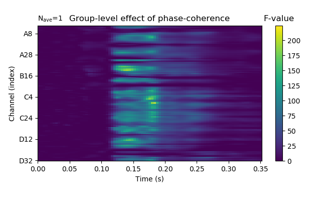
# plot t-values, masking non-significant time points.
fig = group_t['phase-coherence'].plot_image(time_unit='s',
picks=picks,
# mask=sig_mask,
xlim=(0., None),
unit=False,
# keep values scale
scalings=dict(eeg=1),
cmap='viridis',
clim=dict(eeg=[0, None])
)
fig.axes[1].set_title('F-value')
fig.axes[0].set_title('Group-level effect of phase-coherence')
fig.set_size_inches(6.5, 4)
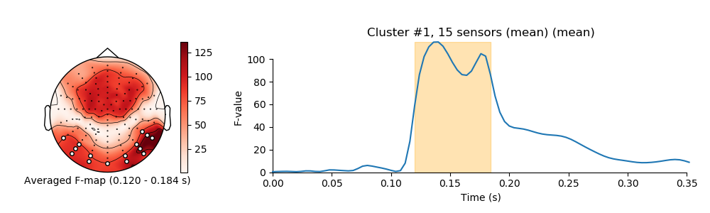
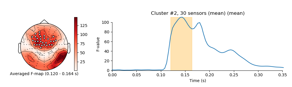
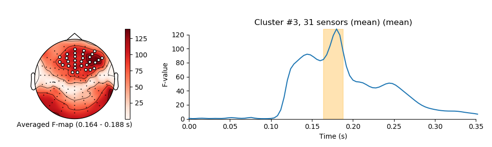
visualize clusters
# get sensor positions via layout
pos = find_layout(epochs_info).pos

# loop over clusters
for i_clu, clu_idx in enumerate(good_cluster_inds):
    # unpack cluster information, get unique indices
    time_inds, space_inds = np.squeeze(clusters[clu_idx])
    ch_inds = np.unique(space_inds)
    time_inds = np.unique(time_inds)

    # get topography for F stat
    f_map = f_vals[time_inds, :].mean(axis=0)

    # get signals at the sensors contributing to the cluster
    sig_times = times[time_inds]

    # create spatial mask
    mask = np.zeros((f_map.shape[0], 1), dtype=bool)
    mask[ch_inds, :] = True

    # initialize figure
    fig, ax_topo = plt.subplots(1, 1, figsize=(10, 3))

    # plot average test statistic and mark significant sensors
    image, _ = plot_topomap(f_map, pos, mask=mask, axes=ax_topo, cmap='Reds',
                            vmin=np.min, vmax=np.max, show=False)

    # create additional axes (for ERF and colorbar)
    divider = make_axes_locatable(ax_topo)

    # add axes for colorbar
    ax_colorbar = divider.append_axes('right', size='5%', pad=0.05)
    plt.colorbar(image, cax=ax_colorbar)
    ax_topo.set_xlabel(
        'Averaged F-map ({:0.3f} - {:0.3f} s)'.format(*sig_times[[0, -1]]))

    # add new axis for time courses and plot time courses
    ax_signals = divider.append_axes('right', size='300%', pad=1.2)
    title = 'Cluster #{0}, {1} sensor'.format(i_clu + 1, len(ch_inds))
    if len(ch_inds) > 1:
        title += "s (mean)"

    plot_compare_evokeds(group_t['phase-coherence-scaled'],
                         title=title,
                         picks=ch_inds,
                         combine='mean',
                         axes=ax_signals,
                         show=False,
                         split_legend=True,
                         truncate_yaxis='max_ticks')

    # plot temporal cluster extent
    ymin, ymax = ax_signals.get_ylim()
    ax_signals.fill_betweenx((ymin, ymax), sig_times[0], sig_times[-1],
                             color='orange', alpha=0.3)
    ax_signals.set_ylabel('F-value')

    # clean up viz
    tight_layout(fig=fig)
    fig.subplots_adjust(bottom=.05)
    plt.show()
Out:
/home/josealanis/Documents/github/mne-stats/examples/group_level/plot_spatiotemporal_cluster.py:337: DeprecationWarning: truncate_yaxis="max_ticks" changed to truncate_yaxis="auto" in version 0.19; in version 0.20 passing "max_ticks" will result in an error. Please update your code accordingly.
  truncate_yaxis='max_ticks')
combining channels using "mean"
/home/josealanis/anaconda3/lib/python3.7/site-packages/matplotlib/figure.py:445: UserWarning: Matplotlib is currently using agg, which is a non-GUI backend, so cannot show the figure.
  % get_backend())
Total running time of the script: ( 0 minutes 48.309 seconds)