Note
Click here to download the full example code
Plot group-level effect of continuous variable
# Authors: Jose C. Garcia Alanis <alanis.jcg@gmail.com>
#
# License: BSD (3-clause)

import numpy as np
from sklearn.linear_model import LinearRegression

import matplotlib.pyplot as plt

from mne.stats.parametric import ttest_1samp_no_p
from mne.datasets import limo
from mne.decoding import Vectorizer, get_coef
from mne.evoked import EvokedArray
from mne import combine_evoked

from mne.viz import plot_compare_evokeds
Here, we’ll import multiple subjects from the LIMO-dataset and explore the group-level beta-coefficients for a continuous predictor.
# list with subjects ids that should be imported
subjects = range(1, 19)
# create a dictionary containing participants data for easy slicing
limo_epochs = {str(subj): limo.load_data(subject=subj) for subj in subjects}

# interpolate missing channels
for subject in limo_epochs.values():
    subject.interpolate_bads(reset_bads=True)
    # only keep eeg channels
    subject.pick_types(eeg=True)
Out:
1055 matching events found
No baseline correction applied
Adding metadata with 2 columns
0 projection items activated
0 bad epochs dropped
1052 matching events found
No baseline correction applied
Adding metadata with 2 columns
0 projection items activated
0 bad epochs dropped
1072 matching events found
No baseline correction applied
Adding metadata with 2 columns
0 projection items activated
0 bad epochs dropped
1050 matching events found
No baseline correction applied
Adding metadata with 2 columns
0 projection items activated
0 bad epochs dropped
1118 matching events found
No baseline correction applied
Adding metadata with 2 columns
0 projection items activated
0 bad epochs dropped
1108 matching events found
No baseline correction applied
Adding metadata with 2 columns
0 projection items activated
0 bad epochs dropped
1060 matching events found
No baseline correction applied
Adding metadata with 2 columns
0 projection items activated
0 bad epochs dropped
1030 matching events found
No baseline correction applied
Adding metadata with 2 columns
0 projection items activated
0 bad epochs dropped
1059 matching events found
No baseline correction applied
Adding metadata with 2 columns
0 projection items activated
0 bad epochs dropped
1038 matching events found
No baseline correction applied
Adding metadata with 2 columns
0 projection items activated
0 bad epochs dropped
1029 matching events found
No baseline correction applied
Adding metadata with 2 columns
0 projection items activated
0 bad epochs dropped
943 matching events found
No baseline correction applied
Adding metadata with 2 columns
0 projection items activated
0 bad epochs dropped
1108 matching events found
No baseline correction applied
Adding metadata with 2 columns
0 projection items activated
0 bad epochs dropped
998 matching events found
No baseline correction applied
Adding metadata with 2 columns
0 projection items activated
0 bad epochs dropped
1076 matching events found
No baseline correction applied
Adding metadata with 2 columns
0 projection items activated
0 bad epochs dropped
1061 matching events found
No baseline correction applied
Adding metadata with 2 columns
0 projection items activated
0 bad epochs dropped
1098 matching events found
No baseline correction applied
Adding metadata with 2 columns
0 projection items activated
0 bad epochs dropped
1103 matching events found
No baseline correction applied
Adding metadata with 2 columns
0 projection items activated
0 bad epochs dropped
Computing interpolation matrix from 113 sensor positions
Interpolating 15 sensors
Computing interpolation matrix from 117 sensor positions
Interpolating 11 sensors
Computing interpolation matrix from 121 sensor positions
Interpolating 7 sensors
Computing interpolation matrix from 119 sensor positions
Interpolating 9 sensors
Computing interpolation matrix from 122 sensor positions
Interpolating 6 sensors
Computing interpolation matrix from 118 sensor positions
Interpolating 10 sensors
Computing interpolation matrix from 117 sensor positions
Interpolating 11 sensors
Computing interpolation matrix from 117 sensor positions
Interpolating 11 sensors
Computing interpolation matrix from 121 sensor positions
Interpolating 7 sensors
Computing interpolation matrix from 116 sensor positions
Interpolating 12 sensors
/home/josealanis/Documents/github/mne-stats/examples/group_level/plot_group_level_effects.py:36: RuntimeWarning: No bad channels to interpolate. Doing nothing...
  subject.interpolate_bads(reset_bads=True)
Computing interpolation matrix from 115 sensor positions
Interpolating 13 sensors
Computing interpolation matrix from 122 sensor positions
Interpolating 6 sensors
Computing interpolation matrix from 114 sensor positions
Interpolating 14 sensors
Computing interpolation matrix from 117 sensor positions
Interpolating 11 sensors
Computing interpolation matrix from 125 sensor positions
Interpolating 3 sensors
Computing interpolation matrix from 126 sensor positions
Interpolating 2 sensors
Computing interpolation matrix from 122 sensor positions
Interpolating 6 sensors
regression parameters
# variables to be used in the analysis (i.e., predictors)
predictors = ['intercept', 'face a - face b', 'phase-coherence']

# number of predictors
n_predictors = len(predictors)

# save epochs information (needed for creating a homologous
# epochs object containing linear regression result)
epochs_info = limo_epochs[str(subjects[0])].info

# number of channels and number of time points in each epoch
# we'll use this information later to bring the results of the
# the linear regression algorithm into an eeg-like format
# (i.e., channels x times points)
n_channels = len(epochs_info['ch_names'])
n_times = len(limo_epochs[str(subjects[0])].times)

# also save times first time-point in data
times = limo_epochs[str(subjects[0])].times
tmin = limo_epochs[str(subjects[0])].tmin
create empty objects for the storage of results
# place holders for bootstrap samples
betas = np.zeros((len(limo_epochs.values()),
                  n_channels * n_times))

# dicts for results evoked-objects
betas_evoked = dict()
t_evokeds = dict()
run regression analysis for each subject
# loop through subjects, set up and fit linear model
for iteration, subject in enumerate(limo_epochs.values()):

    # --- 1) create design matrix ---
    # use epochs metadata
    design = subject.metadata.copy()

    # add intercept (constant) to design matrix
    design = design.assign(intercept=1)

    # effect code contrast for categorical variable (i.e., condition a vs. b)
    design['face a - face b'] = np.where(design['face'] == 'A', 1, -1)

    # order columns of design matrix
    design = design[predictors]

    # column of betas array (i.e., predictor) to run bootstrap on
    pred_col = predictors.index('phase-coherence')

    # --- 2) vectorize (eeg-channel) data for linear regression analysis ---
    # data to be analysed
    data = subject.get_data()

    # vectorize data across channels
    Y = Vectorizer().fit_transform(data)

    # --- 3) fit linear model with sklearn's LinearRegression ---
    # we already have an intercept column in the design matrix,
    # thus we'll call LinearRegression with fit_intercept=False
    linear_model = LinearRegression(fit_intercept=False)
    linear_model.fit(design, Y)

    # --- 4) extract the resulting coefficients (i.e., betas) ---
    # extract betas
    coefs = get_coef(linear_model, 'coef_')
    # only keep relevant predictor
    betas[iteration, :] = coefs[:, pred_col]

    # the matrix of coefficients has a shape of number of observations in
    # the vertorized channel data by number of predictors;
    # thus, we can loop through the columns i.e., the predictors)
    # of the coefficient matrix and extract coefficients for each predictor
    # in order to project them back to a channels x time points space.
    lm_betas = dict()

    # extract coefficients
    beta = betas[iteration, :]
    # back projection to channels x time points
    beta = beta.reshape((n_channels, n_times))
    # create evoked object containing the back projected coefficients
    lm_betas['phase-coherence'] = EvokedArray(beta, epochs_info, tmin)

    # save results
    betas_evoked[str(subjects[iteration])] = lm_betas

    # clean up
    del linear_model
compute mean beta-coefficient for predictor phase-coherence
# subject ids
subjects = [str(subj) for subj in subjects]

# extract phase-coherence betas for each subject
phase_coherence = [betas_evoked[subj]['phase-coherence'] for subj in subjects]

# average phase-coherence betas
weights = np.repeat(1 / len(phase_coherence), len(phase_coherence))
ga_phase_coherence = combine_evoked(phase_coherence, weights=weights)
compute bootstrap confidence interval for phase-coherence betas and t-values
# set random state for replication
random_state = 42
random = np.random.RandomState(random_state)

# number of random samples
boot = 2000

# place holders for bootstrap samples
boot_betas = np.zeros((boot, n_channels * n_times))
boot_t = np.zeros((boot, n_channels * n_times))

# run bootstrap for regression coefficients
for i in range(boot):
    # extract random subjects from overall sample
    resampled_subjects = random.choice(range(betas.shape[0]),
                                       betas.shape[0],
                                       replace=True)
    # resampled betas
    resampled_betas = betas[resampled_subjects, :]

    # compute standard error of bootstrap sample
    se = resampled_betas.std(axis=0) / np.sqrt(resampled_betas.shape[0])

    # center re-sampled betas around zero
    for subj_ind in range(resampled_betas.shape[0]):
        resampled_betas[subj_ind, :] = resampled_betas[subj_ind, :] - \
                                       betas.mean(axis=0)

    # compute t-values for bootstrap sample
    boot_t[i, :] = resampled_betas.mean(axis=0) / se
compute robust CI based on bootstrap-t technique
# compute low and high percentiles for bootstrapped t-values
lower_t, upper_t = np.quantile(boot_t, [.025, .975], axis=0)

# compute group-level standard error based on subjects beta coefficients
betas_se = betas.std(axis=0) / np.sqrt(betas.shape[0])
# lower bound of CI
lower_b = betas.mean(axis=0) - upper_t * betas_se
# upper bound of CI
upper_b = betas.mean(axis=0) - lower_t * betas_se

# reshape to channels * time-points space
lower_b = lower_b.reshape((n_channels, n_times))
upper_b = upper_b.reshape((n_channels, n_times))

# reshape to channels * time-points space
lower_t = lower_t.reshape((n_channels, n_times))
upper_t = upper_t.reshape((n_channels, n_times))
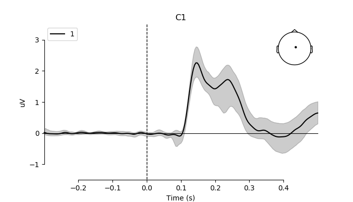
plot mean beta parameter for phase coherence and 95% confidence interval for the electrode showing the strongest effect (i.e., C1)
# index of C1 in array
electrode = 'C1'
pick = ga_phase_coherence.ch_names.index(electrode)

# create figure
fig, ax = plt.subplots(figsize=(7, 4))
plot_compare_evokeds(ga_phase_coherence,
                     ylim=dict(eeg=[-1.5, 3.5]),
                     picks=pick,
                     show_sensors='upper right',
                     colors=['k'],
                     axes=ax)
ax.fill_between(times,
                # transform values to microvolt
                upper_b[pick] * 1e6,
                lower_b[pick] * 1e6,
                color=['k'],
                alpha=0.2)
plt.plot()
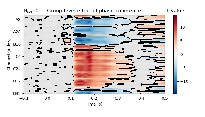
compute one sample t-test on phase coherence betas
# estimate t-values
t_vals = ttest_1samp_no_p(betas)
# back projection to channels x time points
t_vals = t_vals.reshape((n_channels, n_times))

# create mask for "significant" t-values (i.e., above or below
# boot-t quantiles
t_pos = t_vals > upper_t
t_neg = t_vals < lower_t
sig_mask = t_pos | t_neg

# create evoked object containing the resulting t-values
group_t = dict()
group_t['phase-coherence'] = EvokedArray(t_vals, epochs_info, tmin)

# electrodes to plot (reverse order to be compatible whit LIMO paper)
picks = group_t['phase-coherence'].ch_names[::-1]
# plot t-values, masking non-significant time points.
fig = group_t['phase-coherence'].plot_image(time_unit='s',
                                            picks=picks,
                                            mask=sig_mask,
                                            xlim=(-.1, None),
                                            unit=False,
                                            # keep values scale
                                            scalings=dict(eeg=1))
fig.axes[1].set_title('T-value')
fig.axes[0].set_title('Group-level effect of phase-coherence')
fig.set_size_inches(7, 4)
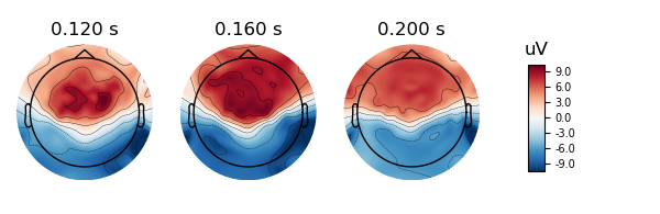
plot topo-map for n170 effect
fig = group_t['phase-coherence'].plot_topomap(times=[.12, .16, .20],
                                              scalings=dict(eeg=1),
                                              sensors=False,
                                              outlines='skirt')
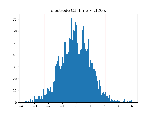
plot t-histograms for n170 effect showing CI boundaries
# times to plot
time_ind_160 = (times > .159) & (times < .161)

# at ~ .120 seconds
plt.hist(boot_t.reshape((boot_t.shape[0],
                         n_channels,
                         n_times))[:, pick, time_ind_160], bins=100)
plt.axvline(x=lower_t[pick, time_ind_160], color='r')
plt.axvline(x=upper_t[pick, time_ind_160], color='r')
plt.title('electrode %s, time ~ .120 s' % electrode)
Total running time of the script: ( 1 minutes 2.041 seconds)