Note
Click here to download the full example code
Plot group-level effect of continuous covariate
# Authors: Jose C. Garcia Alanis <alanis.jcg@gmail.com>
#
# License: BSD (3-clause)

import numpy as np
from pandas import DataFrame
from sklearn.linear_model import LinearRegression
from sklearn.metrics import r2_score
from scipy.stats import zscore

import matplotlib.pyplot as plt

from mne.datasets import limo
from mne.decoding import Vectorizer, get_coef
from mne.evoked import EvokedArray

from mne.viz import plot_compare_evokeds
Here, we’ll import multiple subjects from the LIMO-dataset and use this data to explore the modulating effects of subjects age on the phase-coherence. i.e., how the effect of phase-coherence varied across subjects as a function of their age. Here we’ll create a data frame containing the age values for second-level analysis, but a copy of the data frame can be found as .tsv on the to directory of mne-limo.
# subject ids
subjects = range(1, 19)
# create a dictionary containing participants data for easy slicing
limo_epochs = {str(subj): limo.load_data(subject=subj) for subj in subjects}

# interpolate missing channels
for subject in limo_epochs.values():
    subject.interpolate_bads(reset_bads=True)
    # only keep eeg channels
    subject.pick_types(eeg=True)

# subjects age
age = [66, 68, 37, 68, 32, 21, 60, 68, 37, 28, 68, 41, 32, 34, 60, 61, 21, 40]
subj_age = DataFrame(data=age,
                     columns=['age'])
Out:
1055 matching events found
No baseline correction applied
Adding metadata with 2 columns
0 projection items activated
0 bad epochs dropped
1052 matching events found
No baseline correction applied
Adding metadata with 2 columns
0 projection items activated
0 bad epochs dropped
1072 matching events found
No baseline correction applied
Adding metadata with 2 columns
0 projection items activated
0 bad epochs dropped
1050 matching events found
No baseline correction applied
Adding metadata with 2 columns
0 projection items activated
0 bad epochs dropped
1118 matching events found
No baseline correction applied
Adding metadata with 2 columns
0 projection items activated
0 bad epochs dropped
1108 matching events found
No baseline correction applied
Adding metadata with 2 columns
0 projection items activated
0 bad epochs dropped
1060 matching events found
No baseline correction applied
Adding metadata with 2 columns
0 projection items activated
0 bad epochs dropped
1030 matching events found
No baseline correction applied
Adding metadata with 2 columns
0 projection items activated
0 bad epochs dropped
1059 matching events found
No baseline correction applied
Adding metadata with 2 columns
0 projection items activated
0 bad epochs dropped
1038 matching events found
No baseline correction applied
Adding metadata with 2 columns
0 projection items activated
0 bad epochs dropped
1029 matching events found
No baseline correction applied
Adding metadata with 2 columns
0 projection items activated
0 bad epochs dropped
943 matching events found
No baseline correction applied
Adding metadata with 2 columns
0 projection items activated
0 bad epochs dropped
1108 matching events found
No baseline correction applied
Adding metadata with 2 columns
0 projection items activated
0 bad epochs dropped
998 matching events found
No baseline correction applied
Adding metadata with 2 columns
0 projection items activated
0 bad epochs dropped
1076 matching events found
No baseline correction applied
Adding metadata with 2 columns
0 projection items activated
0 bad epochs dropped
1061 matching events found
No baseline correction applied
Adding metadata with 2 columns
0 projection items activated
0 bad epochs dropped
1098 matching events found
No baseline correction applied
Adding metadata with 2 columns
0 projection items activated
0 bad epochs dropped
1103 matching events found
No baseline correction applied
Adding metadata with 2 columns
0 projection items activated
0 bad epochs dropped
Computing interpolation matrix from 113 sensor positions
Interpolating 15 sensors
Computing interpolation matrix from 117 sensor positions
Interpolating 11 sensors
Computing interpolation matrix from 121 sensor positions
Interpolating 7 sensors
Computing interpolation matrix from 119 sensor positions
Interpolating 9 sensors
Computing interpolation matrix from 122 sensor positions
Interpolating 6 sensors
Computing interpolation matrix from 118 sensor positions
Interpolating 10 sensors
Computing interpolation matrix from 117 sensor positions
Interpolating 11 sensors
Computing interpolation matrix from 117 sensor positions
Interpolating 11 sensors
Computing interpolation matrix from 121 sensor positions
Interpolating 7 sensors
Computing interpolation matrix from 116 sensor positions
Interpolating 12 sensors
/home/josealanis/Documents/github/mne-stats/examples/group_level/plot_continuous_covariate.py:40: RuntimeWarning: No bad channels to interpolate. Doing nothing...
  subject.interpolate_bads(reset_bads=True)
Computing interpolation matrix from 115 sensor positions
Interpolating 13 sensors
Computing interpolation matrix from 122 sensor positions
Interpolating 6 sensors
Computing interpolation matrix from 114 sensor positions
Interpolating 14 sensors
Computing interpolation matrix from 117 sensor positions
Interpolating 11 sensors
Computing interpolation matrix from 125 sensor positions
Interpolating 3 sensors
Computing interpolation matrix from 126 sensor positions
Interpolating 2 sensors
Computing interpolation matrix from 122 sensor positions
Interpolating 6 sensors
regression parameters
# variables to be used in the analysis (i.e., predictors)
predictors = ['intercept', 'face a - face b', 'phase-coherence']

# number of predictors
n_predictors = len(predictors)

# save epochs information (needed for creating a homologous
# epochs object containing linear regression result)
epochs_info = limo_epochs[str(subjects[0])].info

# number of channels and number of time points in each epoch
# we'll use this information later to bring the results of the
# the linear regression algorithm into an eeg-like format
# (i.e., channels x times points)
n_channels = len(epochs_info['ch_names'])
n_times = len(limo_epochs[str(subjects[0])].times)

# also save times first time-point in data
times = limo_epochs[str(subjects[0])].times
tmin = limo_epochs[str(subjects[0])].tmin
create empty objects for the storage of results
run regression analysis for each subject
# loop through subjects, set up and fit linear model
for iteration, subject in enumerate(limo_epochs.values()):

    # --- 1) create design matrix ---
    # use epochs metadata
    design = subject.metadata.copy()

    # add intercept (constant) to design matrix
    design = design.assign(intercept=1)

    # effect code contrast for categorical variable (i.e., condition a vs. b)
    design['face a - face b'] = np.where(design['face'] == 'A', 1, -1)

    # order columns of design matrix
    design = design[predictors]

    # column of betas array (i.e., predictor) to run bootstrap on
    pred_col = predictors.index('phase-coherence')

    # --- 2) vectorize (eeg-channel) data for linear regression analysis ---
    # data to be analysed
    data = subject.get_data()

    # vectorize data across channels
    Y = Vectorizer().fit_transform(data)

    # --- 3) fit linear model with sklearn's LinearRegression ---
    # we already have an intercept column in the design matrix,
    # thus we'll call LinearRegression with fit_intercept=False
    linear_model = LinearRegression(fit_intercept=False)
    linear_model.fit(design, Y)

    # --- 4) extract the resulting coefficients (i.e., betas) ---
    # extract betas
    coefs = get_coef(linear_model, 'coef_')
    # only keep relevant predictor
    betas[iteration, :] = coefs[:, pred_col]

    # calculate coefficient of determination (r-squared)
    r_squared[iteration, :] = r2_score(Y, linear_model.predict(design),
                                       multioutput='raw_values')

    # clean up
    del linear_model
create design matrix from group-level regression
# z-core age predictor
subj_age['age'] = zscore(subj_age['age'])
# create design matrix
group_design = subj_age

# add intercept
group_design = group_design.assign(intercept=1)
# order columns of design matrix
group_predictors = ['intercept', 'age']
group_design = group_design[group_predictors]

# column index of relevant predictor
group_pred_col = group_predictors.index('age')
run bootstrap for group-level regression coefficients
# set random state for replication
random_state = 42
random = np.random.RandomState(random_state)

# number of random samples
boot = 2000

# create empty array for saving the bootstrap samples
boot_betas = np.zeros((boot, n_channels * n_times))
# run bootstrap for regression coefficients
for i in range(boot):
    # extract random subjects from overall sample
    resampled_subjects = random.choice(range(betas.shape[0]),
                                       betas.shape[0],
                                       replace=True)

    # resampled betas
    resampled_betas = betas[resampled_subjects, :]

    # set up model and fit model
    model_boot = LinearRegression(fit_intercept=False)
    model_boot.fit(X=group_design.iloc[resampled_subjects], y=resampled_betas)

    # extract regression coefficients
    group_coefs = get_coef(model_boot, 'coef_')

    # store regression coefficient for age covariate
    boot_betas[i, :] = group_coefs[:, group_pred_col]

    # delete the previously fitted model
    del model_boot
compute CI boundaries according to: Pernet, C. R., Chauveau, N., Gaspar, C., & Rousselet, G. A. (2011). LIMO EEG: a toolbox for hierarchical LInear MOdeling of ElectroEncephaloGraphic data. Computational intelligence and neuroscience, 2011, 3.
# a = (alpha * number of bootstraps) / (2 * number of predictors)
a = (0.05 * boot) / (2 / group_pred_col * 1)
# c = number of bootstraps - a
c = boot - a

# compute low and high percentiles for bootstrapped beta coefficients
lower_b, upper_b = np.quantile(boot_betas, [a/boot, c/boot], axis=0)

# reshape to channels * time-points space
lower_b = lower_b.reshape((n_channels, n_times))
upper_b = upper_b.reshape((n_channels, n_times))
fit linear model with sklearn’s LinearRegression we already have an intercept column in the design matrix, thus we’ll call LinearRegression with fit_intercept=False
# set up and fit model
linear_model = LinearRegression(fit_intercept=False)
linear_model.fit(group_design, betas)

# extract group-level beta coefficients
group_coefs = get_coef(linear_model, 'coef_')

# only keep relevant predictor
group_betas = group_coefs[:, group_pred_col]

# back projection to channels x time points
group_betas = group_betas.reshape((n_channels, n_times))
# create evoked object containing the back projected coefficients
group_betas_evoked = EvokedArray(group_betas, epochs_info, tmin)
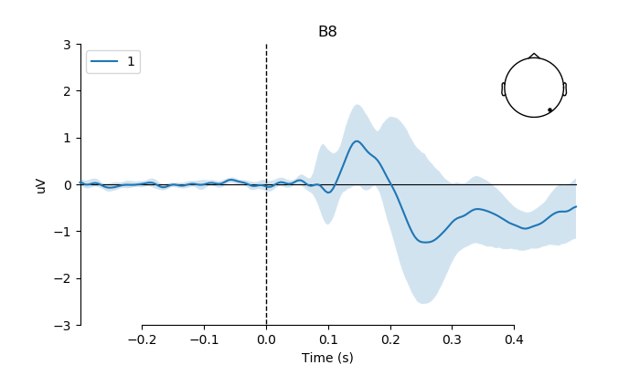
plot the modulating effect of age on the phase coherence predictor (i.e., how the effect of phase coherence varies as a function of subject age) using whole electrode montage and whole scalp by taking the same physical electrodes across subjects
# index of B8 in array
electrode = 'B8'
pick = group_betas_evoked.ch_names.index(electrode)

# create figure
fig, ax = plt.subplots(figsize=(7, 4))
ax = plot_compare_evokeds(group_betas_evoked,
                          ylim=dict(eeg=[-3, 3]),
                          picks=pick,
                          show_sensors='upper right',
                          axes=ax)
ax[0].axes[0].fill_between(times,
                           # transform values to microvolt
                           upper_b[pick] * 1e6,
                           lower_b[pick] * 1e6,
                           alpha=0.2)
plt.plot()
run analysis on optimized electrode (i.e., electrode showing best fit for phase-coherence predictor).
# find R-squared peak for each subject in the data set
optimized_electrodes = r_squared.argmax(axis=1)
# find the corresponding electrode
optimized_electrodes = np.unravel_index(optimized_electrodes,
                                        (n_channels, n_times))[0]
extract beta coefficients for electrode showing best fit
# reshape subjects' beats to channels * time-points space
betas = betas.reshape((betas.shape[0], n_channels, n_times))

# get betas for best fitting electrode
optimized_betas = np.array(
    [subj[elec, :] for subj, elec in zip(betas, optimized_electrodes)])
fit linear model with sklearn’s LinearRegression
linear_model = LinearRegression(fit_intercept=False)
linear_model.fit(group_design, optimized_betas)

# extract group-level beta coefficients
group_opt_coefs = get_coef(linear_model, 'coef_')

# only keep relevant predictor
group_pred_col = group_predictors.index('age')
group_opt_betas = group_opt_coefs[:, group_pred_col]
run bootstrap for group-level regression coefficients derived from optimized electrode analyisis
# set random state for replication
random_state = 42
random = np.random.RandomState(random_state)

# number of random samples
boot = 2000

# create empty array for saving the bootstrap samples
boot_optimized_betas = np.zeros((boot, n_times))
# run bootstrap for regression coefficients
for i in range(boot):
    # extract random subjects from overall sample
    resampled_subjects = random.choice(range(betas.shape[0]),
                                       betas.shape[0],
                                       replace=True)

    # resampled betas
    resampled_betas = optimized_betas[resampled_subjects, :]

    # set up model and fit model
    model_boot = LinearRegression(fit_intercept=False)
    model_boot.fit(X=group_design.iloc[resampled_subjects], y=resampled_betas)

    # extract regression coefficients
    group_opt_coefs = get_coef(model_boot, 'coef_')

    # store regression coefficient for age covariate
    boot_optimized_betas[i, :] = group_opt_coefs[:, group_pred_col]

    # delete the previously fitted model
    del model_boot
compute CI boundaries according to: Pernet, C. R., Chauveau, N., Gaspar, C., & Rousselet, G. A. (2011). LIMO EEG: a toolbox for hierarchical LInear MOdeling of ElectroEncephaloGraphic data. Computational intelligence and neuroscience, 2011, 3.
# a = (alpha * number of bootstraps) / (2 * number of predictors)
a = (0.05 * boot) / (2 / group_pred_col * 1)
# c = number of bootstraps - a
c = boot - a

# or compute with np.quantile
# compute low and high percentiles for bootstrapped beta coefficients
lower_ob, upper_ob = np.quantile(boot_optimized_betas, [a/boot, c/boot], axis=0)
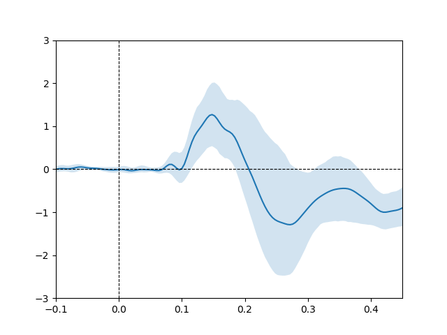
plot the modulating effect of age on the phase coherence predictor for optimized electrode
# create figure
plt.plot(times, group_opt_betas * 1e6)  # transform betas to microvolt
plt.fill_between(times,
                 # transform values to microvolt
                 lower_ob * 1e6,
                 upper_ob * 1e6,
                 alpha=0.2)
plt.axhline(y=0, ls='--', lw=0.8, c='k')
plt.axvline(x=0, ls='--', lw=0.8, c='k')
plt.ylim(top=3, bottom=-3)
plt.xlim(-.1, .45)
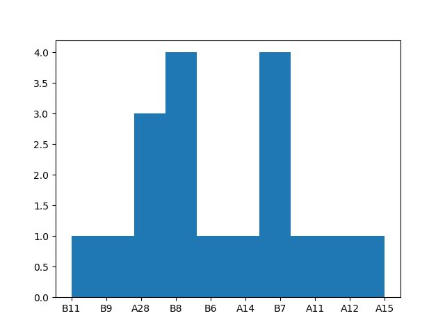
plot histogram of optimized electrode frequencies
electrode_freq = [limo_epochs['1'].ch_names[e] for e in optimized_electrodes]
plt.hist(electrode_freq)
Total running time of the script: ( 1 minutes 12.565 seconds)